目录
0 前言 在此前的文章《最小二乘法多项式曲线拟合数学原理及其 C++ 实现》 中,我们给出了标准最小二乘法用于多项式拟合的数学原理推导及其 C++ 代码实现。
应用标准最小二乘法拟合多项式时,我们认为各个样本点的权重是相同的,即每个样本点对总的拟合误差的贡献是相同的,但在工程应用中,有时需要为样本点赋予不同的权重,即我们允许最终的拟合结果在更加贴合某些高权重样本点的基础上偏离某些低权重样本点。
本文将在前文的基础上给出加权最小二乘多项式拟合的数学推导及其 C++ 实现。
1 符号约定 本文中对所使用数学符号所做的约定与前文相同:
简体小写字母:标量。例如,$s$、$\theta_0$。注意,本文中的微分符号 $d$ 也使用简体小写字母
粗体小写字母:向量。例如,$\boldsymbol{\theta}$、$\mathbf{y}$、$\mathbf{y_r}$
粗体大写字母:矩阵。例如,$\mathbf{X}$、$\mathbf{X_v}$
2 数学推导 我们已经知道,最小二乘法通过最小化误差的平方和寻找数据的最优函数匹配。给定一组样本数据集 $P(x, y)$,$P$ 内各数据点 $P_i(x_i, y_i) (i=1, 2, 3, …, m)$ 来自于对多项式
的多次采样,其中:
$m$ 为样本维度
$n$ 为多项式阶数
$\theta_j (j=0,1, 2, …, n)$ 为多项式的各项系数
与标准最小二乘法不同的是,这里我们为每个数据点 $P_i(x_i, y_i) (i=1, 2, 3, …, m)$ 定义一个正权重因子 $w_i$,则样本数据集 $P$ 内各数据点的加权误差平方和 $s_w$ 为:
加权最小二乘法认为,最优函数的各项系数 $\theta_j$ 应使得加权误差平方和 $s_w$ 取得极小值。我们令
则加权误差平方和 $s_w$ 可写成:
其中,$\mathbf{X_v}$ 是由样本数据集的输入构造的范德蒙矩阵,$\mathbf{W}$ 是由样本数据集中各个数据点的权重因子构造的权重对角矩阵,$\boldsymbol{\theta}$ 是多项式系数构成的系数向量,$\mathbf{y_r}$ 是样本数据集的输出向量。对于最优函数,应满足:
注意,式 (2.5) 中的 $\mathbf{0}$ 为向量。$\frac{\partial{s_w}}{\partial{\boldsymbol{\theta}}}$ 是标量对向量的导数,这里我们不直接推导它,而是从推导 $s_w$ 的微分 $ds_w$ 开始:
式 (2.6) 的推导与《最小二乘法多项式曲线拟合数学原理及其 C++ 实现》 中式 (3.9) 的推导类似,此处不再赘述。
$s_w$ 是关于 $\theta_j (j=0,1, 2, …, n)$ 的多元函数,我们知道多元函数的全微分公式为:
联立式 (2.6) 和式 (2.7):
联立式 (2.5) 和式 (2.8),很容易求得最优函数的多项式系数向量 $\boldsymbol{\theta}$:
观察式 (2.9) 的结果我们不难发现,加权最小二乘多项式拟合的结果与标准最小二乘形式差别不大。
3 代码实现 本文中使用 C++ Eigen 库对加权最小二乘法多项式拟合进行了实现,并在 Ubuntu 20.04 下进行了测试验证,使用 Python matplotlib 库对拟合结果进行了可视化,完整 C++ 工程可点击这里 进行下载,工程目录结构说明如下:
1
2
3
4
5
6
7
8
9
10
11
___ ├── bin // 可执行文件存放目录 ├── build // 工程构建目录 ├── build.sh // 工程构建脚本,被 run.sh 调用 ├── CMakeLists.txt // cmake 描述文件 ├── data // 原始数据及拟合结果存放目录 ├── inc // 头文件目录 ├── main.cpp // 程序入口文件 ├── plot.py // 原始数据及拟合结果可视化脚本 ├── run.sh // 可执行程序运行脚本,将自动调用 build.sh 完成工程构建 └── src // 源文件目录
通过执行工程根目录下的 run.sh 脚本将自动完成工程编译与运行,运行结果将存放在工程根目录的 data 目录下。
3.1 加权最小二乘多项式拟合实现 a. 函数声明
下述代码段来自 inc/weighted_least_square.hpp:
1 2 3 4 5 6 7 8 9 10 11 12 13 14 15 16 17 18 19 20 21 22 23 24 #ifndef WEIGHTED_LEAST_SQUARE_HPP_ #define WEIGHTED_LEAST_SQUARE_HPP_ #include <vector> #include <Eigen/Dense> struct Point2D { float x = 0.0f ; float y = 0.0f ; float weight = 1.0f ; Point2D(float param_x, float param_y, float param_weight) { x = param_x; y = param_y; weight = param_weight; } }; std::pair<bool, Eigen::VectorXf> WeightedLeastSquare( const std ::vector <Point2D>& points, uint8_t orders); #endif
这里我们自定义了 Point2D 数据结构用于表示带权重属性的 2D 点,WeightedLeastSquare 函数有两个形参:
points:待拟合的原始数据点orders:待拟合的多项式阶数
b. 函数实现
下述代码段来自 src/weighted_least_square.cpp:
1 2 3 4 5 6 7 8 9 10 11 12 13 14 15 16 17 18 19 20 21 22 23 24 25 26 27 28 29 30 31 32 33 34 35 36 37 38 39 40 41 42 43 44 45 46 47 48 49 50 51 52 53 54 55 56 57 58 59 60 61 62 63 64 65 #include <iostream> #include "../inc/weighted_least_square.hpp" std::pair<bool, Eigen::VectorXf> WeightedLeastSquare( const std ::vector <Point2D>& points, uint8_t orders) { auto samples_num = points.size(); std ::pair<bool , Eigen::VectorXf> failure_result{false , Eigen::VectorXf()}; if (samples_num < orders + 1 || orders < 1 ) { std ::cout << "Insufficient sampling points to fit a " << orders << " order polynomial, please check it!" << std ::endl ; return failure_result; } Eigen::VectorXf sample_x (samples_num) ; Eigen::VectorXf sample_y (samples_num) ; Eigen::MatrixXf weight_mtx (samples_num, samples_num) ; float weight_sum = 0.0f , weight_sum_epsilon = 1E-6 f; for (size_t i = 0 ; i < samples_num; ++i) { if (points.at(i).weight < 0.0f ) { std ::cout << "Invalid weight " << points.at(i).weight << " of point " << i << ", please check it!" << std ::endl ; return failure_result; } sample_x(i) = points.at(i).x; sample_y(i) = points.at(i).y; weight_sum += points.at(i).weight; } if (weight_sum > weight_sum_epsilon) { for (size_t i = 0 ; i < samples_num; ++i) weight_mtx(i, i) = points.at(i).weight / weight_sum; } else { std ::cout << "The total weight " << weight_sum << " is too small, please check it!" << std ::endl ; return failure_result; } Eigen::MatrixXf vandermonde_mtx (samples_num, orders + 1 ) ; vandermonde_mtx.col(0 ) = Eigen::VectorXf::Constant(samples_num, 1 , 1 ); for (size_t i = 1 ; i < orders + 1 ; ++i) { vandermonde_mtx.col(i) = vandermonde_mtx.col(i - 1 ).array () * sample_x.array (); } Eigen::MatrixXf tmp = vandermonde_mtx.transpose() * weight_mtx; Eigen::VectorXf coeffs = (tmp * vandermonde_mtx).inverse() * tmp * sample_y; return {true , coeffs}; }
WeightedLeastSquare 函数的实现主要包含四个步骤:
步骤 1:数据预处理。将原始数据点的横纵坐标分别读入 Eigen 列向量,并计算所有数据点的总权重
步骤 2:权重归一化
步骤 3:逐列构造范德蒙矩阵
步骤 4:求解多项式系数
实现细节与前文中的数学推导章节相对应,此处不再赘述。
3.2 测试与验证 下述代码段来自 main.cpp:
1 2 3 4 5 6 7 8 9 10 11 12 13 14 15 16 17 18 19 20 21 22 23 24 25 26 27 28 29 30 31 32 33 34 35 36 37 38 39 40 41 42 43 44 45 46 47 48 49 50 51 52 53 54 55 56 57 58 59 60 61 62 63 64 65 66 67 68 69 70 71 72 73 74 75 76 #include <iostream> #include <string> #include <fstream> #include <random> #include "inc/weighted_least_square.hpp" std ::vector <Point2D> GenData () std ::ofstream fs; fs.open("../data/raw_data.txt" , std ::fstream::app); std ::default_random_engine e; std ::uniform_real_distribution<float > u (-500.0f , 500.0f ) size_t points_num = 50 ; std ::vector <Point2D> points; points.reserve(points_num); for (float x = 1 ; x <= static_cast <float >(points_num); ++x) { float y = 4 + 3 * x + 1.2f * std ::pow (x, 2 ) - 0.001f * std ::pow (x, 3 ) + u(e); points.emplace_back(x, y, 1.0f ); fs << x << " " << y; if (x < points_num) fs << std ::endl ; } fs.close(); return points; } void FitData (const std ::vector <Point2D>& points, const std ::string & file_name) std ::ofstream fs; auto result = WeightedLeastSquare(points, 3 ); if (result.first) { const auto & coeffs = result.second; std ::string file_path = "../data/" + file_name; fs.open(file_path, std ::fstream::app); fs << coeffs(0 ) << " " << coeffs(1 ) << " " << coeffs(2 ) << " " << coeffs(3 ); fs.close(); } } int main () auto points = GenData(); for (size_t i = 0 ; i < points.size(); ++i) { points.at(i).weight = 1.0f ; } FitData(points, "standard_least_square.txt" ); for (size_t i = 0 ; i < points.size(); ++i) { points.at(i).weight = i < points.size() / 2 ? 100.0f : 0.5f ; } FitData(points, "weighted_least_square_1.txt" ); for (size_t i = 0 ; i < points.size(); ++i) { points.at(i).weight = i >= points.size() / 2 ? 100.0f : 0.5f ; } FitData(points, "weighted_least_square_2.txt" ); return 0 ; }
这里我们首先通过基函数
以及在 $[-500.0, 500.0]$ 区间上服从均匀分布的随机数生成了 50 个待拟合的原始数据点,然后通过调节数据点的权重进行了三组拟合测试:
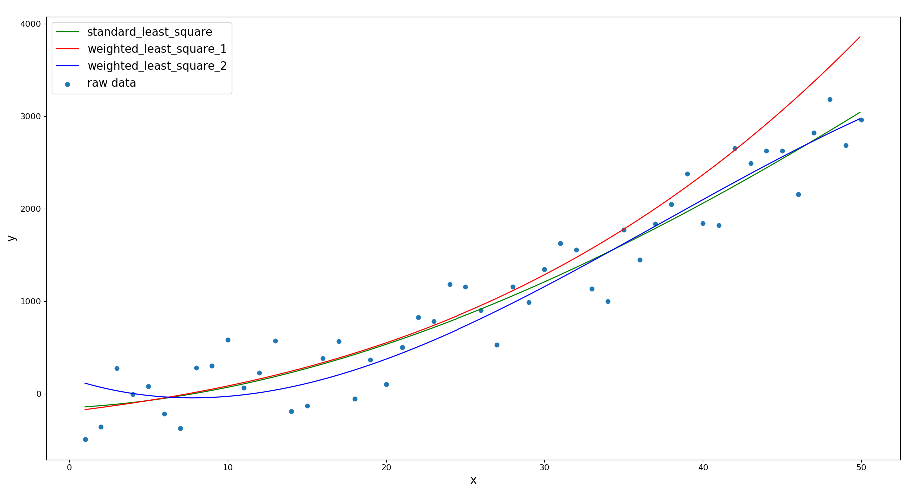
标准最小二乘拟合:所有数据点都拥有相同的权重
加权最小二乘拟合 1:前半部分数据点的权重更高
加权最小二乘拟合 2:后半部分数据点的权重更高
通过执行工程根目录下的 run.sh 脚本完成工程编译与运行后,原始数据点以及三组拟合结果将分别存放在工程根目录的 data 目录下的对应 .txt 文本文件中。由于数据量较少,最终拟合得到的多项式与式 (3.1) 可能差别较大,这是正常现象。
通过执行工程根目录下的 plot.py 脚本,绘制原始数据点及拟合结果:
从上图中我们可以发现:
调高前半部分数据点的权重时,拟合得到的多项式曲线与原始数据点后半部分存在较大偏差
调高后半部分数据点的权重时,拟合得到的多项式曲线与原始数据点前半部分存在较大偏差
结果符合预期。
参考
最小二乘法多项式曲线拟合数学原理及其 C++ 实现